Chapter 6 Multilevel Models
6.1 Contextual Backgorund
What are multilevel models?
Multilevel models (MLMs) are mathematical summaries of nested data structures, or data structures that contain (at least the potential for) extra dependence.
What do you mean by ‘extra dependence’?
Well, normally when we perform regression analysis (see Chapter 5), we assume that each of the individuals within the data set is independent from the others. For example, within the education data set used within Chapter 5, we assumed that the score of one child is not related to the score of another child. Why assume independence between subjects? Because the mathematical computation underlying regression is much simpler if we can assume independence, and in many cases the assumption can be theoretically (i.e., practically) justified. However, there are cases where it is very likely that our subjects are not independent, and for those instances we need to be certain that we model (i.e., account for) that dependence.
Can you give an example when independence isn’t justified?
Certainly. The classic example comes from the field of education. Imagine that you are a researcher studying students’ mathematics ability. You collect students’ scores on a mathemtics test across several classrooms within a school. At first you think that you should run a simple regression analysis, something like \[math_i = b_0 + b_1 \cdot covar_i + \epsilon_i \]
but then you begin to wonder whether you have violated the independence assumption that is embedded within a regression analysis. In particular, you’ve heard that some teachers are better than other teachers, and that may cause some classrooms to perform better on the mathematics test.
Let’s consider two different scenarios. Scenario 1: some teachers perform better than others; Scenario 2: teachers are about the same. We depict the likely outcomes of the two scenarios below.
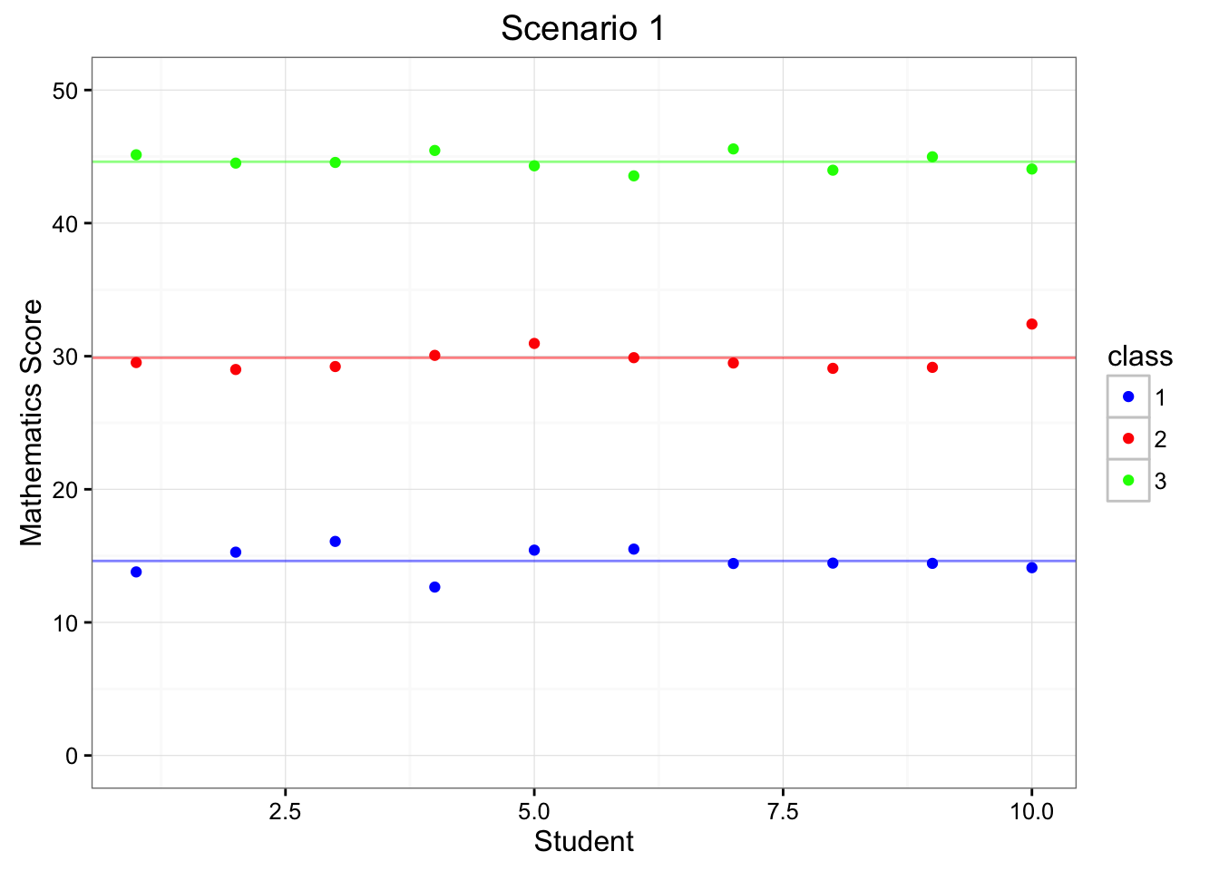
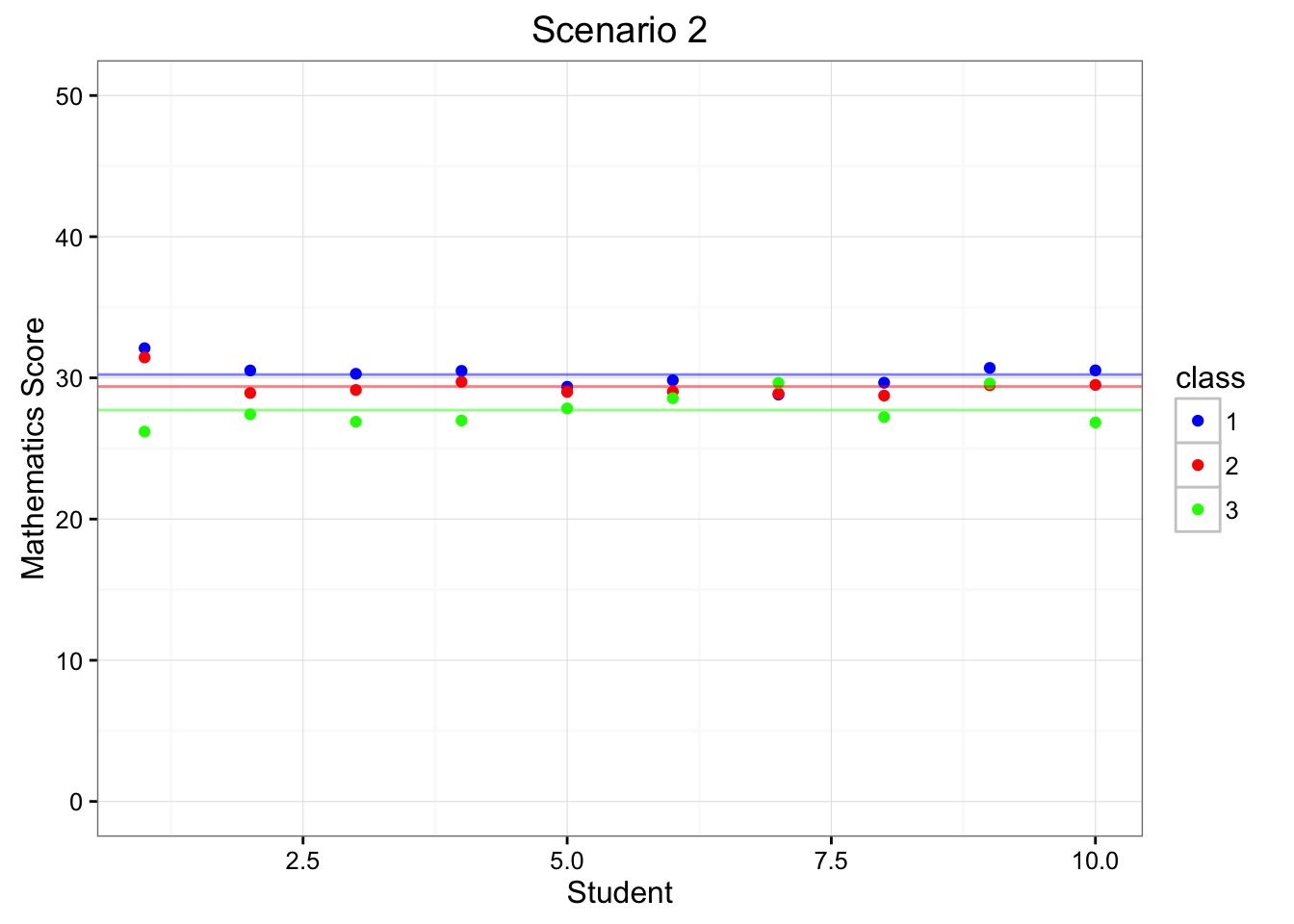
Figure 6.1: Depiction of Scenarios 1 & 2
Figure 6.1 depicts the mathematics test scores (y-axis) of 10 individuals (x-axis) for three different classrooms (1, 2, 3; colored as blue, red, and green). The horizonal lines portray each classroom’s average test score. Within Scenario 1 (left-hand side of Figure 6.1), each of the classrooms have very different means, indicating that the teachers have different effects on the children within each of their respective classrooms. On the other hand, Scenario 2 (right-hand side of Figure 6.1) indicates that teachers have similar effects on children as they score very similarly across classrooms.
Within Scenario 1 there is an extra level of dependence. We can see that if we know which classroom you are in, then we know something about how you will perform on the mathematics exam. Stated differently, the scores within a classroom are much more related (i.e. dependent) than scores across the classrooms.
Alternatively, Scenario 2 does not have an extra level of dependence. We can see that the mathematics scores didn’t systematically vary according to the classroom.
Hence, multilevel models are used when we can see that there are sub-groups of individuals, and that the responses of individuals within those sub-groups have dependence (i.e., tend to have a similar pattern). Sometimes we refer to this data structure as nested, such that students are nested within classrooms.
This all sounds very similar to hierarchical linear models. How are multilevel models different from hierarchical linear models?
Actually, they aren’t different at all. They are different names for the same modeling approach. To be more specific, multilevel models, hierarchical linear models, random coefficient models, and mixed effects models are all the same. The truth is that these different individuals contributed to the identification and estimation of these models, and as they were built they each provided their own name for the method.
For some reason I always thought that multilevel models were only for longitudinal data. Can they be used for longitudinal data?
Absolutely. We can reconstruct Figure 6.1 to be a longitudinal example rather than a cross-sectional example. In particular, we can have 10 observations for three people, and the information within the Figure would stay the same:
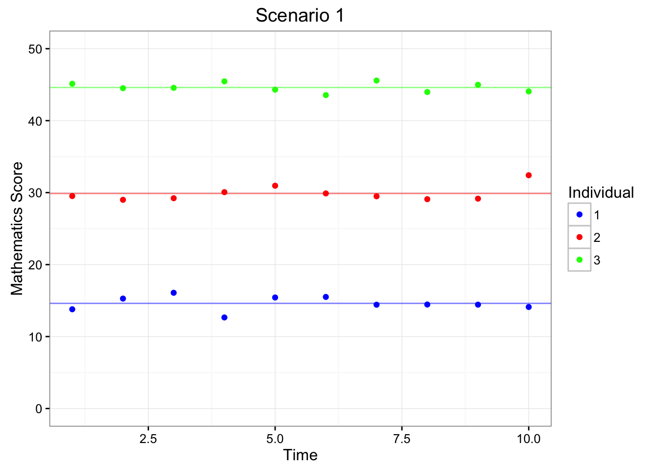
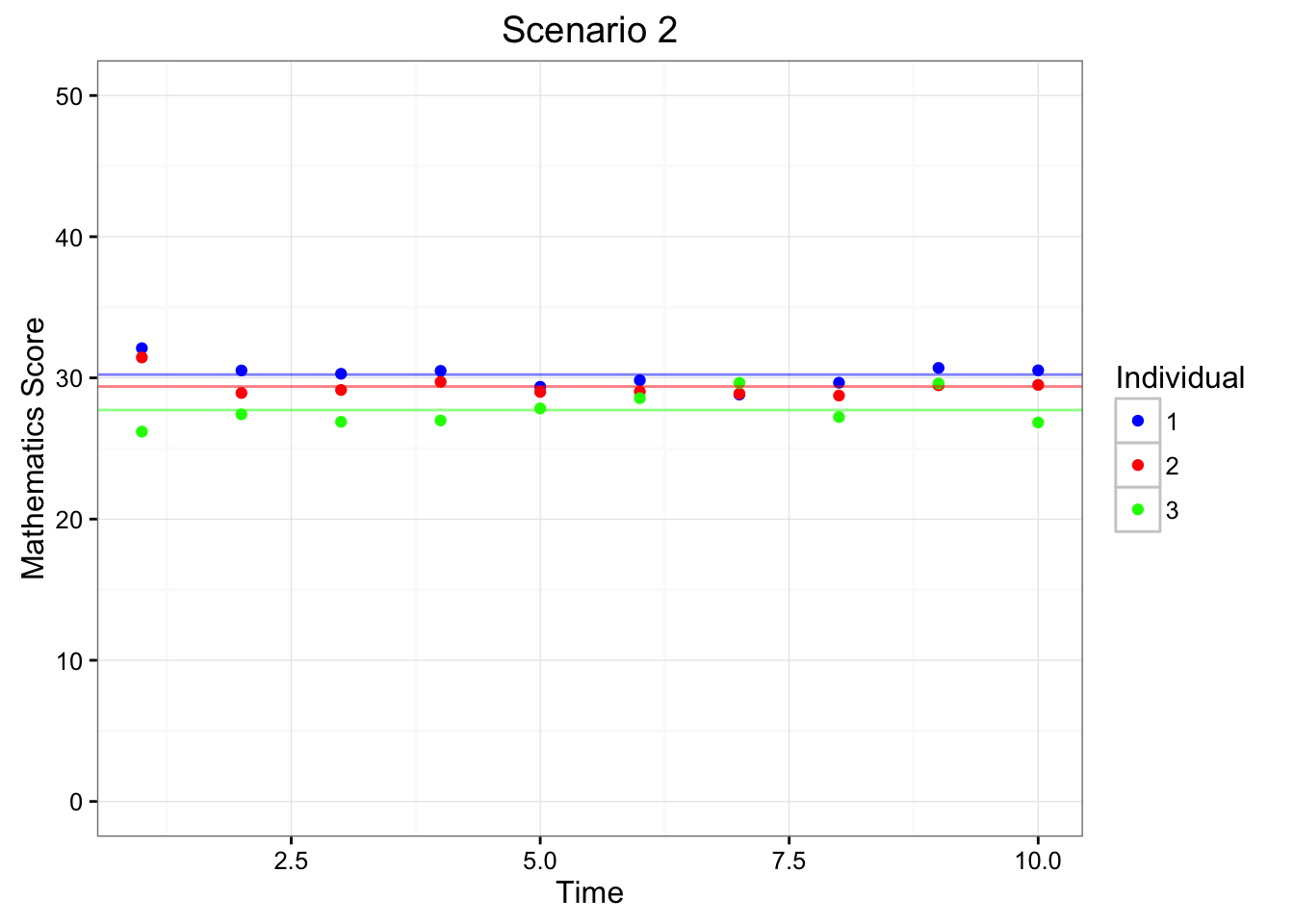
Figure 6.2: Depiction of Scenarios 1 & 2 Using Longitudinal Data
Figure 6.2 depicts the mathematics test scores (y-axis) of across 10 measurement occassions (x-axis) for three different individuals (1, 2, 3; colored as blue, red, and green). The horizonal lines portray each individual’s average test score. Within Scenario 1 (left-hand side of Figure 6.2), each of the individuals have very different means, indicating that they have different overall mathematics abilities. On the other hand, Scenario 2 (right-hand side of Figure 6.1) indicates that indiviudals tend to have similar mathematics abilities across repeated measures.
Ok, so how exactly do we account for (i.e, model) this dependence?
Let’s cover that in the next sub-section of this chapter.
6.2 Concepts of MLMs
Ok, so how exactly do we account for (i.e, model) this dependence?
Let’s talk about the mathematical concepts of MLMs first, and then we’ll talk more about the modeling strategy. Conceptually, multilevel models account for the dependence by allowing each group (i.e., different classrooms from the cross-sectional example, and different individuals from the longitudinal example) to have their own regression equation.
For example, we could have three different regression equations for Scenario 1 of either the cross-sectional or longitudinal examples. More specifically, we would have
For classroom = 1: \(y_{1i} = b_{01} + \epsilon_{1i}\)
For classroom = 2: \(y_{2i} = b_{02} + \epsilon_{2i}\)
For classroom = 3: \(y_{3i} = b_{03} + \epsilon_{3i}\)
where \(i\) refers to a specific individual within a classroom; \(b_{01}\), \(b_{02}\), and \(b_{03}\) represent the mean scores within each of the classrooms; and \(\epsilon_{i1}\), \(\epsilon_{i2}\), \(\epsilon_{i3}\) indicate the remaining portion of \(y_{i1}\), \(y_{i2}\), and \(y_{i3}\) unaccounted for by \(b_{01}\), \(b_{02}\), and \(b_{03}\).
Using this nomenclature, we can comnense the three equations above into a single equation:
For classroom \(c\): \(y_{ci} = b_{0c} + \epsilon_{ci}\)
Of course, it is important to note that the condensed equation may also be used for the longitudinal example. Rather that having individuals within classrooms, we have observations within individuals. This leads to
For individual \(i\): \(y_{it} = b_{0i} + \epsilon_{it}\)
Then, by using either the cross-sectional or longitudinal model, we assume that the remaining part of the the data (i.e., the residuals: \(\epsilon_{ci}\) or \(\epsilon_{it}\)) are independent. Sometimes we state this is ‘conditional independence’, which is a short-hand way of stating that ‘the observations are independent conditioned on the model’, or ‘the residuals are independent after we have accounted for the dependence using the \(b_{0c}\) or the \(b_{0i}\).’
To give an example of ‘conditional independence’, consider Figure 6.3:
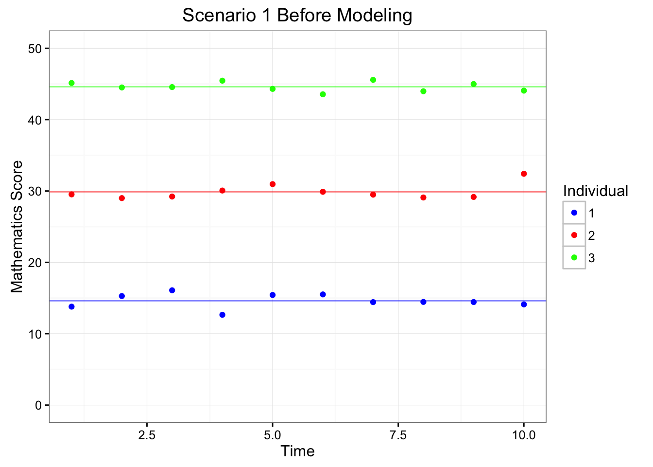
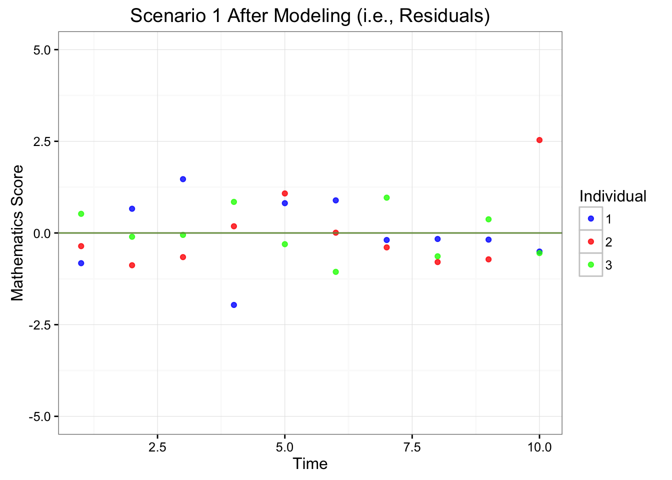
Figure 6.3: Depiction of Scenarios 1 Before and After Modeling
Within the second panel of Figure 6.3, we can see that each of the individuals tend to vary around the same mean. Hence, the differences between the individuals become trivial after we have accounted for their respective mean differences (i.e., \(b_{01}\), \(b_{02}\), and \(b_{03}\)). Therefore, we have accounted for the dependence using the model.
So is that all MLMs are? Just separate regressions for each of the groups?
Not exactly, but don’t groan too loudly. Conceptually, MLMs are just separate regressions for each of the groups. But we need to do more than just run separate regressions, and we’ll talk about that in the next sub-section.
6.3 Why Not Run Separate Regressions?
At this stage you may be asking why we don’t run separate regressions for each of the groups. As we have noted in the conceptual section above, this is how we can account for the dependence structure that occurs within nested data. And its relatively simple. So why not?
There are many answers to this question, but here I explain (what I believe) are the two most fundamental reasons. The first has to do with parsimony, and the second has to do with generalizability.
Reason 1: Parsimony In the examples above it was relatively simple to estimate a set of coefficients for each of the classrooms/individuals because there were only three coefficients (i.e., the three intercepts: \(b_{01}\), \(b_{02}\), and \(b_{03}\)). However, if we had 100, or even 1,000 classrooms/individuals the model would require an extremely large number of parameters, making it not a very parsimonious description of the phenomenon.
Reason 2: Generalizability We implement models to provide summaries of a sample that (hopeufully) generalize to the population. For example, if we fit a regular regression model (\(y_i = b_0 + b_1 \cdot covar_i + \epsilon_i\)) to a sample of data, then we describe the results (i.e., we interpret \(b_0\) and \(b_1\)) in the context of the population.
However, in the case of nested data, if we have one coefficient per group (e.g., classroom or individual) then each of the coefficients generalize to a specific group; but none correpsond to the population. Therefore, the model coefficients provide a good summary of each group, but do not tell us much about how the phenomenon manifests within the population.
6.4 Group Level Coefficients as a Distribution
The beauty of MLMs arises from the use of distributions to summarize a set of coefficients across groups. To demonstrate this property, let’s consider the classroom example a second time, but let’s say that we have twenty classrooms instead of three. This could look like:
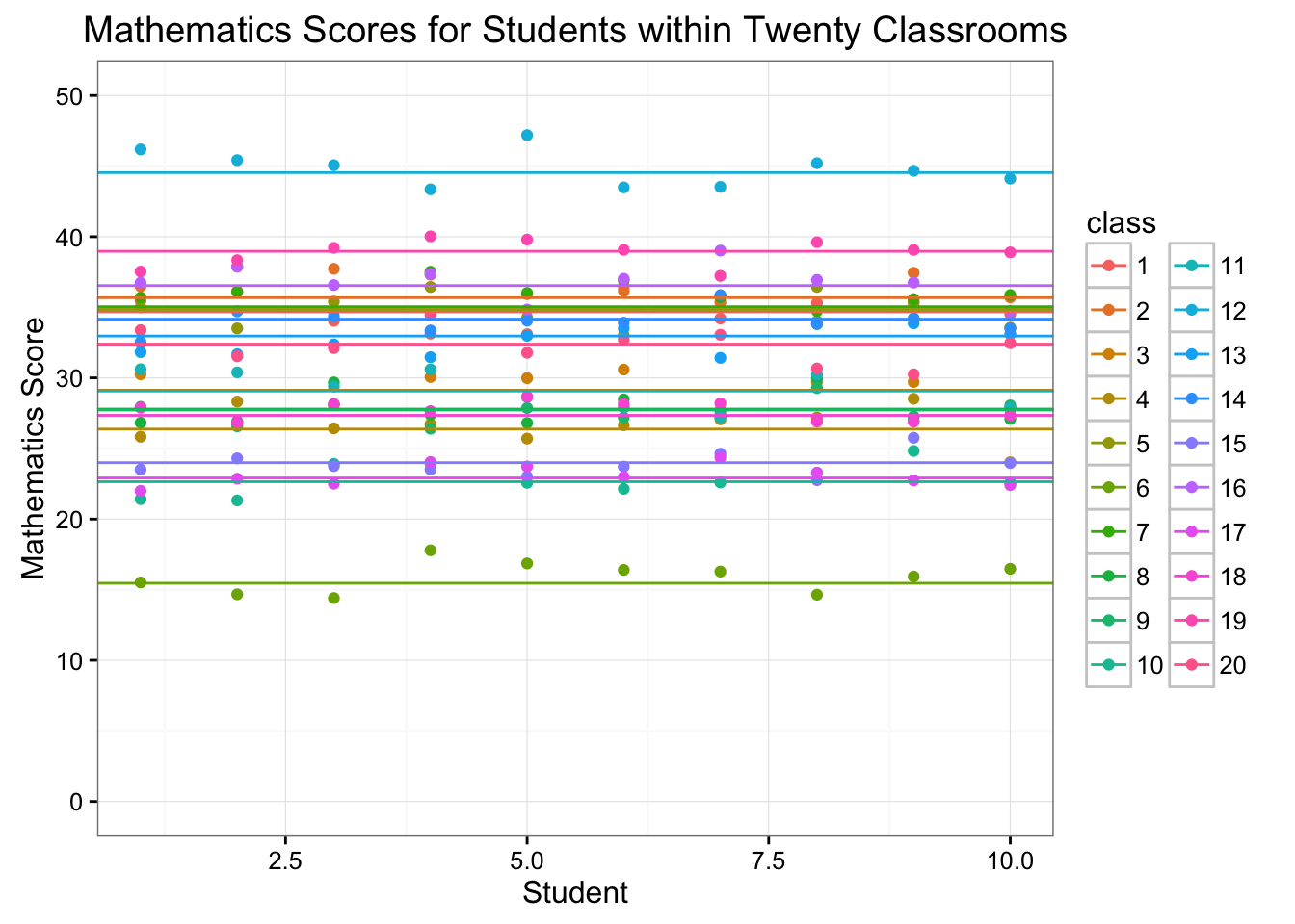
Figure 6.4: Mathematics Scores for Students within Twenty Classrooms
When examining the different means for each classroom (i.e., the horizontal lines within Figure 6.4), we may begin to notice that the \(b_{0c}\) follow a normal distribution. More specifically, we may surmise that \[ b_{0c} \sim N(\mu_{b_0}, \sigma^2_{b_0}) \]
If this assumption holds, then we have solutions to Reasons 1 & 2 from above. First, we no longer need to estimate as many parameters (i.e., coefficients) as we have groups; rather we will only need to estimate the mean (\(\mu_{b_0}\)) and the variance (\(\sigma^2_{b_0}\)). This property holds no matter how many groups we have within our data set, hence we maintain a parsimonious solution regardless of the number of groups.
Second, the parameters that we estimate (\(\mu_{b_0}\) and \(\sigma^2_{b_0}\)) characeterize the population. For example, we could say that we expect students to earn about a mathematics score of \(\mu_{b_0}\), and we expect 95% of the classroom means to be within two standard deviations (i.e., \(\pm2 \cdot\sigma_{b_0}\)).
Therefore, by assuming that the model coefficients follow a particular distribution, we are able to account for the dependence of the nested structure in parsimonious and generalizable manner.
6.5 Computational Estimation of MLMs
I’m not really sure how to estimate MLMs. How does estimation work?
Great question, and an answer that is well beyond the scope of this particular chapter. Most readers are not interested in learning about the technical aspects of parameter estimation, so I will only provide a more conceptual explanation to the estimation approach that underlies MLMs. If enough readers request more technical details, I will provide the information within a future chapter.
Generally, the estimation procedures represent highly sophisticated guess and check algorithms that shift through two different stages. The output of one stage is a current estimate of the group specific coefficients (i.e., the \(b_0c\) or \(b_0i\) from the examples above), whereas the output of the other stage is an estimate of the population parameters of interest (i.e., \(\mu_{b_0}\) and \(\sigma^2_{b_0}\) from the examples above). Each stage uses the output from the previous stage. Thus, estimation of the group specific coefficients are the those that best fit the data given the assumption that the population parameters from the previous stage are correct. And, estimation of the population coefficients are those that best fit the data *given the assumption that the group specific parameters from the previous stage are correct. The algorithm iterates between these two stages, and the parameters change at each step along the way. Eventually, the parameters will change by a trivial amount (i.e., the difference between \(\mu_{b_0}\) and \(\sigma^2_{b_0}\) from on iteration to the next will be less than \(1^{-7}\)), and then estimation ceases.
As a bit of an aside, the mathematical implementation that occurs within each stage differs across estimation suites. Therefore, different software packages may provide slightly different parameter estimates and standard errors. These discrepancies should not be worrisome, unless the parameter estimates provide qualitatively different interpretations (i.e., one method produces a significnatly positive coefficient, and the other a significantly negative coefficient). If strong discrepancies occur, make sure you’re using the same data set and model across the different packages.